
Comprehensive tips for reliable and efficient analysis set-up
Cancer Genomics Cloud
Comprehensive tips for reliable and efficient analysis set-up
Objective
This guide is designed to help you with your first set of projects on the CGC. Each section has specific examples and instructions to demonstrate how to accomplish each step. Also listed are common mistakes to avoid while setting up a project. If you need more information on a particular subject, our Knowledge Center has additional information on all of the features of the CGC. Additionally, our Support Team is available 24/7 to help.
Helpful terms to know
Tool / App (interchangeably used) – refers to a stand-alone bioinformatics tool or its Common Workflow Language (CWL) wrapper that is created or already available on the platform.
Workflow / Pipeline (interchangeably used) – denotes a number of apps connected together in order to perform multiple analysis steps in one run.
Task – represents an execution of a particular app or workflow on the platform. Depending on what is being executed (app or workflow), a single task can consist of only one tool execution (app case) or multiple executions (one or more per each app in the workflow).
Job – this refers to the “execution” part from the “Task” definition (see above). It represents a single run of a single tool found within a workflow. If you are coming from a computer science background, you will notice that the definition is quite similar to a common understanding of the term “job” (wikipedia). Except that the “job” is a component of a bigger unit of work called a “task” and not the other way around, as in some other areas may be the case. To further illustrate what job means on the platform, we can visually inspect jobs after the task has been executed using the View stats & logs panel (button in the upper right corner on the task page):
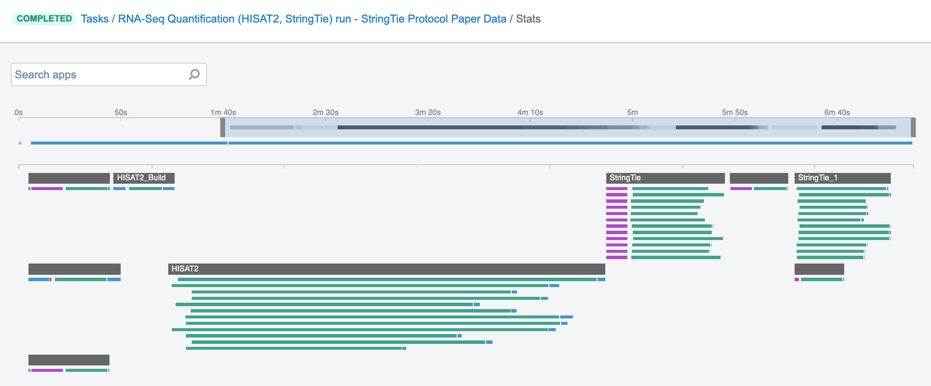
The green bars under the gray ones (apps) represent the jobs (Figure 1). As you can see, some apps (e.g. HISAT2_Build) consist of only one job, whereas others (e.g. HISAT2) contain multiple jobs that are executed simultaneously.
User Accounts & Billing Groups
Setting up a Cancer Genomics Cloud (CGC) account is free of charge - we encourage researchers to register here and try out one of the most advanced genomics analysis environments available.
Upon registration, each user receives $300 in credits in a "Pilot Fund" billing group to get started. Once those credits have been consumed, any user can create a paid billing group that is associated with a credit card or purchase order.
The work on CGC is divided into separate workspaces called projects (Figure 2). Each user can create projects and invite other registered users to be members of those projects. In addition, a variety of permission levels (e.g. admin, write, read-only) can be assigned to each project member.
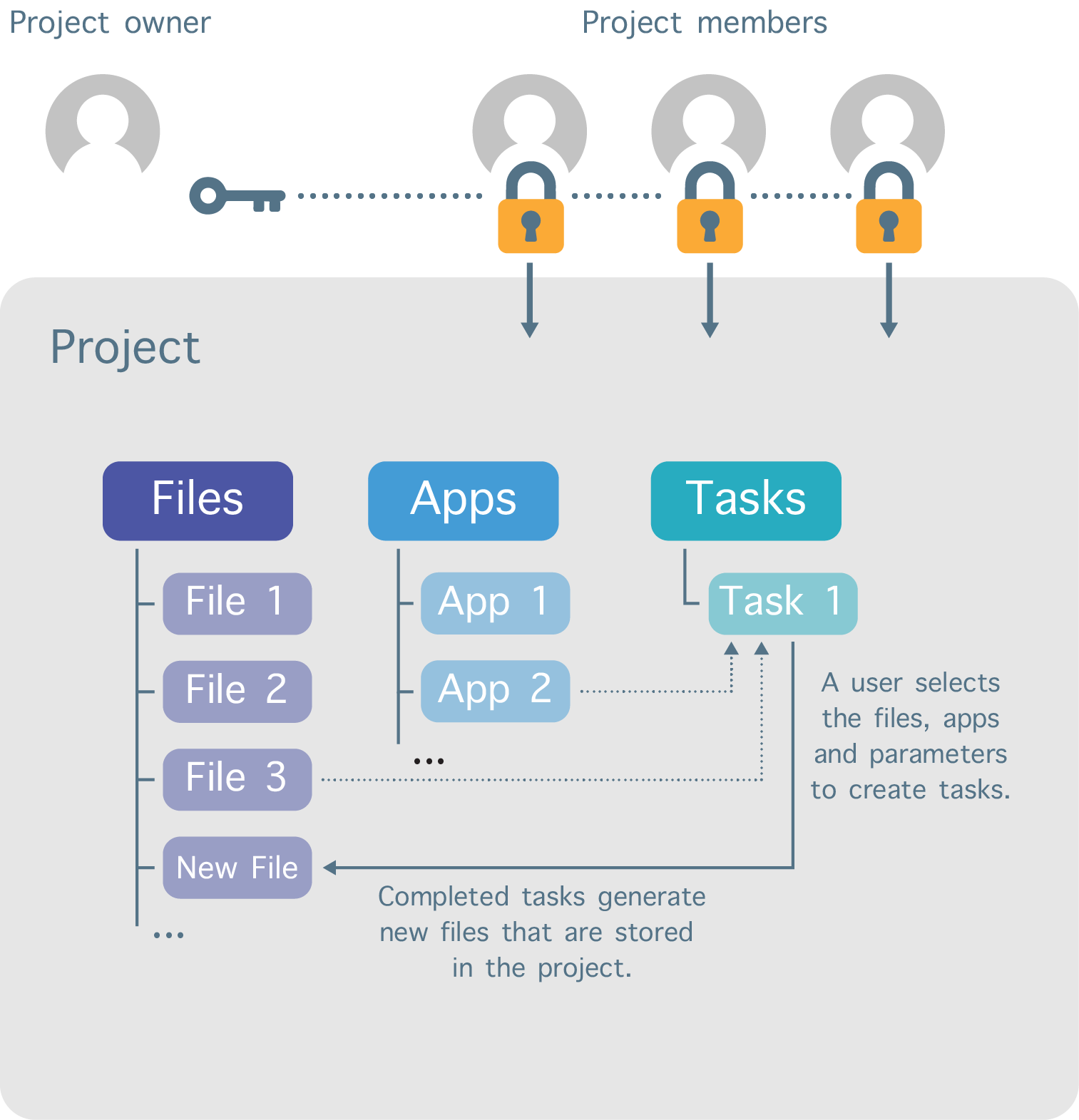
The user that creates the project sets the billing group to which the project’s storage and compute costs are billed, and this billing group can be changed at any time.

Further Reading
Sign up for the CGC:
https://docs.cancergenomicscloud.org/docs/sign-up-for-the-cgc
Before you start:
https://docs.cancergenomicscloud.org/docs
Access via the visual interface:
https://docs.cancergenomicscloud.org/docs/access-via-the-visual-interface
Projects on the CGC:
https://docs.cancergenomicscloud.org/docs/projects-on-the-cgc
Add a collaborator to a project:
https://docs.cancergenomicscloud.org/docs/add-a-collaborator-to-a-project
Change the billing group for a project:
https://docs.cancergenomicscloud.org/docs/modify-project-settings
Account settings and billing:
https://docs.cancergenomicscloud.org/docs/account-settings-and-billing
Tips for Running Apps/Workflows
In this section, you will find some of the most essential information on how to set up and run tools and workflows on the platform. Creating CWL wrappers is not in the scope of this section (for that, see here); instead, we focus on platform features which are fundamental to making your analysis efficient and scalable. The content is structured such that it first offers information that is helpful for those researchers who want to use the public tools and workflows, and then it gradually advances to describe the features which can be used to adjust existing tools or develop new tools.
Start with the descriptions
For users who plan to execute any one of the hundreds of hosted tools or workflows from the CGC Public Apps Gallery, the most important step is to thoroughly read the description. Even if you are familiar with the tools or you regularly run similar tools on your local machine, the description is where you will find the most useful, relevant, and up-to-date information on what you can expect in terms of the analysis design, expected analysis duration, expected cost, common issues, and more. The Common Issues and Important Note section is an essential section in the description which gives insights into the known pitfalls when running the tool and should be studied thoroughly, especially when planning to run large scale analysis.
Although Seven Bridges and the CGC aim to continuously improve the hosted public apps and seek to educate researchers on their proper use, there are many places for error which can cause the tools/workflows to fail to successfully execute. Below is an example of how overlooking the description notes caused an unexpected outcome for a user:
Bioinformatics tools are usually designed to fail if certain inputs are configured incorrectly, and therefore terminate the misconfigured execution as soon as possible. However, in the case of VarDict variant caller, failing to provide the required input index files does not always result in the failure and can sometimes lead to infinite running.
This exact outcome occured when a user tried to process a number of samples by using the VarDict Single Sample Calling workflow. Previously, the user analyzed an entire cohort of samples with this workflow without any issues. Next, the user tried to apply the same strategy to another dataset in a different project. When setting up the workflow in the new project, the user copied the reference files to the new project and initiated the workflow with this new batch of files. However, the user left out the reference genome index file (FAI file) during the copying step, in turn producing several tasks which suffered from infinite running. Since the index files are automatically loaded from the project and not referenced explicitly as separate inputs, it was even more likely for this issue to go unnoticed.
The situation was additionally compounded by having a batch task (see Batch Analysis section for more details) which contained hundreds of children tasks. Because the user was not familiar with the related notes from the workflow description, they were not aware that the running tasks might in fact be hanging tasks. Had they known, they would have been able to terminate the run earlier, saving time and money.
In this case, the majority of the tasks failed early in the execution, producing minimal charges, but a few frozen tasks doubled the costs expected for the entire batch. We have since addressed the issues in this particular tool by introducing additional checks and input validations in the wrapper. Even though this is an extreme example, it demonstrates how descriptions can be critical to your tool working properly and can help you make informed decisions.
Test the workflow
For users planning a large scale analysis, it is recommended to begin by testing the workflow in a small number (1-5) of runs. By testing tools on a small scale, users can quickly make sure that everything works as expected, while minimizing costs. Additionally, testing the pipeline for the worst case scenario is one of the best ways to get more insight into the potential edge cases which could arise. This can often be accomplished by running the analysis with the files of largest size in a given dataset. There are other situations where the highest computational load will correlate with the complexity of the sample content rather than correlating with size, which is more difficult to estimate. Familiarity with the experimental design behind the sample files helps to create proper test cases for both size and complexity, which can keep potential errors to a minimum.
Specify computational resources
The term “computational instance” or “instance” refers to a virtual machine that can be chosen in order to adjust CPU and memory capacities for a particular application. The instances can be selected from the predefined list of Amazon EC2 or Google Cloud instance types.
For public apps, the instance resources have been pre-tested and defined by the CGC team. In most cases, the pre-defined instance types and default parameters will work for the majority of workflows, but users may need to optimize for certain input sizes or complexities, especially when scaling up workflows.
Small-scale testing can help inform if adjustments are needed in regard to the instance type(s) or tool parameters to be used throughout the analysis. There are two means by which instance selection is controlled:
- Resource parameters
- Instance selection
For the public apps and workflows, resource parameters are typically adjustable through the Memory per job and CPU per job parameters. Setting the values for these will cause the scheduling component to allocate the most optimal instance type given these values. The following is an example from the task page:
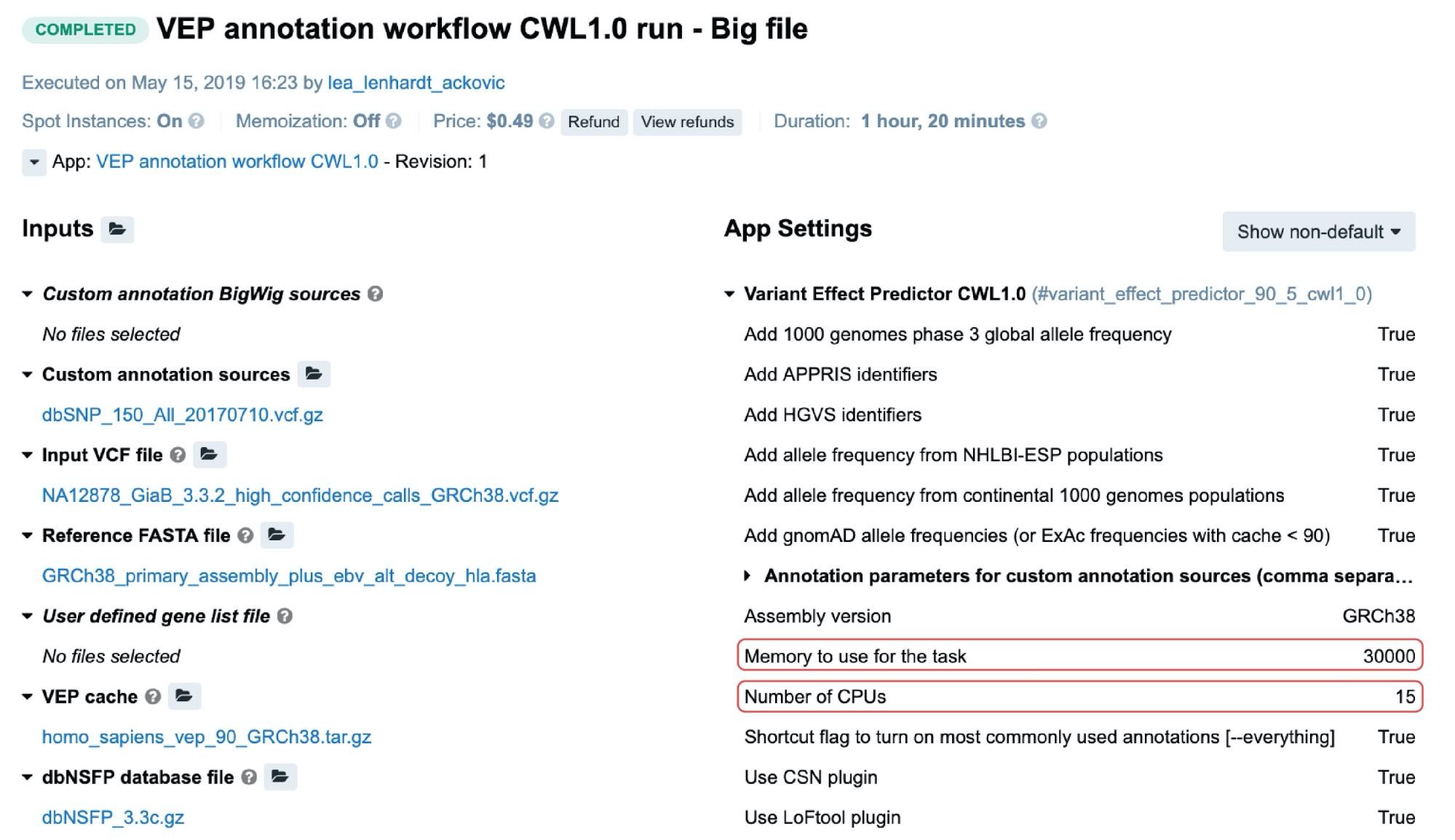
In this particular case, c5.4xlarge instance (32.0 GiB, 16 vCPUs) was automatically allocated based on the two highlighted resource parameters (Figure 3). If we take a moment to examine the other instance types which may fit this requirement, we may note that c4.4xlarge comes with 30.0 GiB and 16 vCPUs, which are the values closer to the given ones. However, the platform’s scheduling component also takes into account the price, and since c5.4xlarge is slightly cheaper than c4.4xlarge it was given precedence.
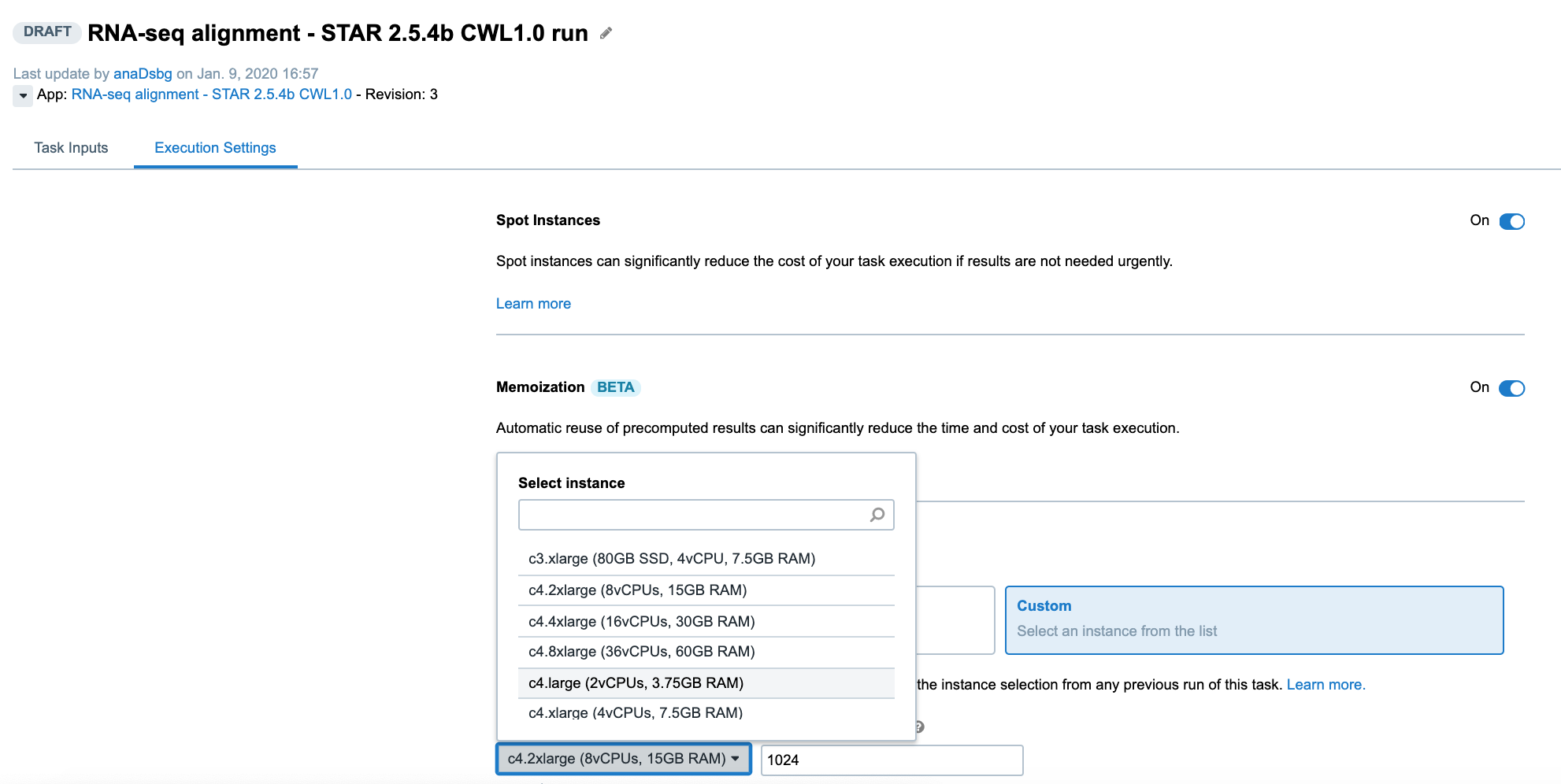
Another way to control the computational resources is to explicitly choose an instance type from the Execution Settings panel on the task page:
Learn about Instance Profiles
To be able to get the most out of available computational resources, it is essential to know how each individual tool behaves in different scenarios, such as when using different input parameters or different data file sizes. One of the most efficient ways to identify patterns that perform well and use them to optimize future analyses is to monitor resource profiles.
The following is an example of the figures accessible from the Instance metrics panel found within stats & logs page (View stats & logs button is located in the upper right corner on the task page):
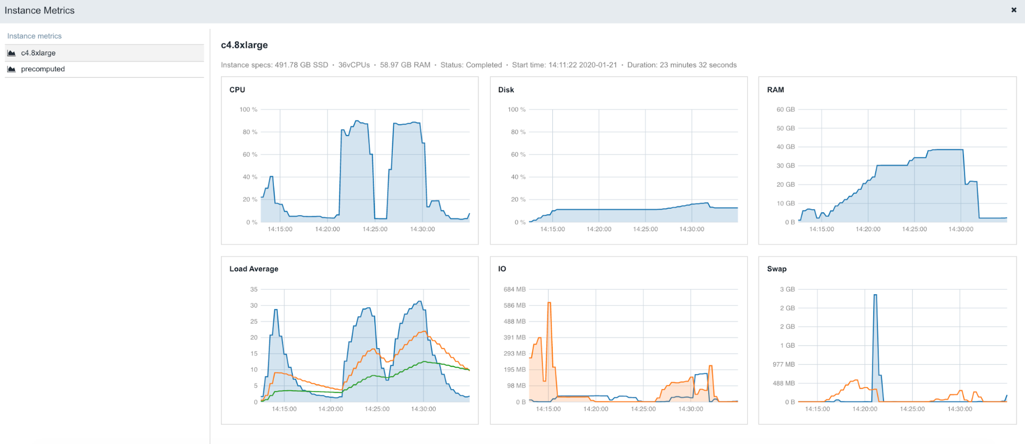
To learn more about Instance metrics, visit the related documentation page in our Knowledge Center.
Scale up with Batch Analysis
Batch analysis is an important step when analyzing larger datasets, typically consisting of many files for which it is desirable to apply the same processing methods throughout. We use batch analysis to create separate, analytically-identical tasks for each given item (either a file or a group of files depending on the batching method).
Two batching modes are available:
- Batch by File
- Batch by File metadata
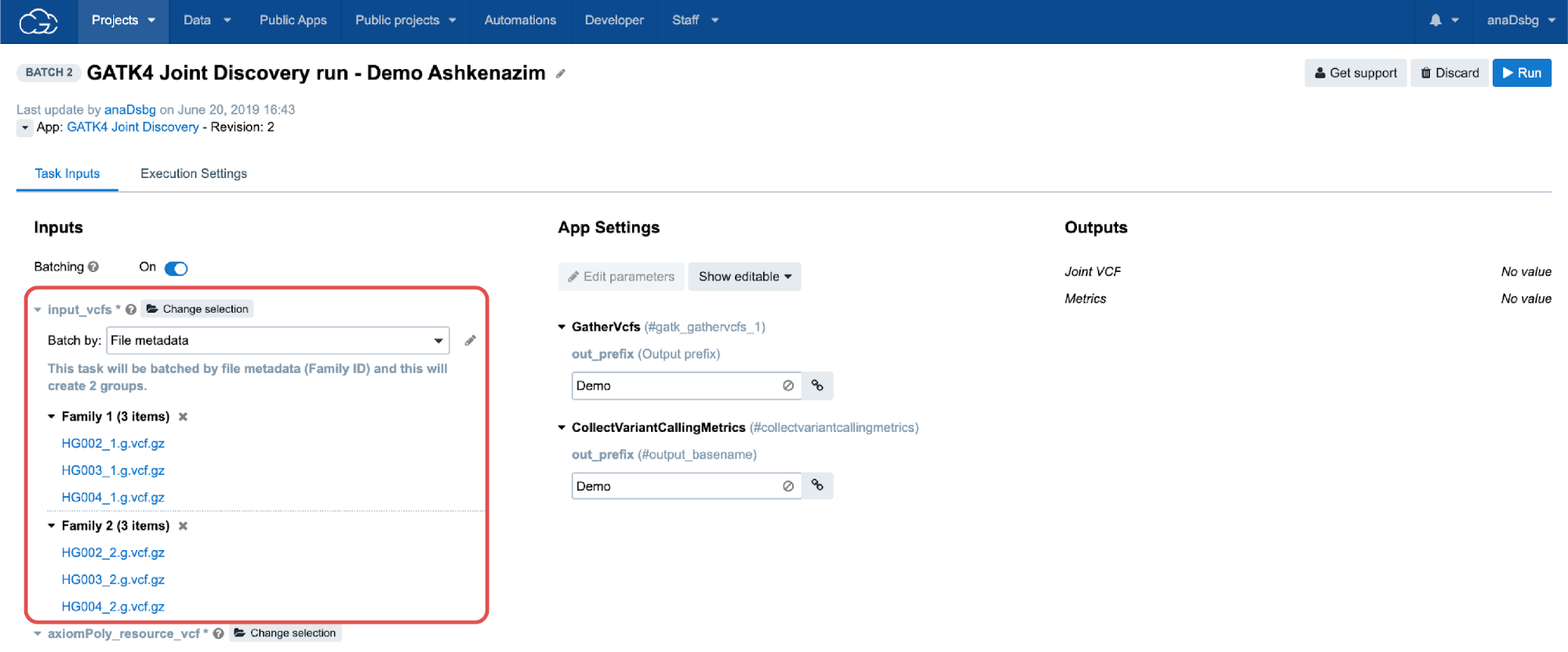
In the Batch by File scenario, a task will be created for each file selected in the batched input. In the Batch by File Metadata scenario, a task will be created for each group of files that correspond to a specified value of the metadata (Figure 6).
Batch analysis is quite robust in regard to errors or failures, meaning that failures in one task will not affect other tasks within the same batch of analysis. In other words, if we process multiple samples using batch analysis, each sample will have its own task. If one task fails, the other tasks will continue to process and can complete successfully, and the analysis will still be able to complete for most samples. Alternatively, it is possible to process multiple samples using another feature called Scatter (described in the following section), and have all the samples processed within a single task. In contrast to batch analysis, a failure of any part of the scatter task (i.e. a job for an individual sample), will cause the entire task to fail and thus the analysis for all samples to also fail. In summary, batch analysis highly simplifies the process of creating a large number of the same tasks while allowing independent, simultaneous executions.
Important: Before starting large scale executions with Batch Analysis, please refer to the “Computational Limits” section below.
Parallelize with Scatter
Many common analyses will benefit from highly parallel executions, such as analyzing groups of files from specific disease types (e.g. TCGA BRCA). The first factor that will determine the parallelization strategy is the user desires to execute the same tool multiple times within one computational instance, or instead to use multiple, independent instances to run the whole analysis in parallel for different input files (i.e. batch analysis). The feature which enables the former is called Scatter.
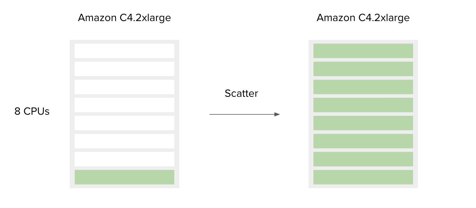
The following is a simple example to accompany Figure 7.
SBG Decompressor is a simple app used for extracting files from compressed bundles. It requires only one CPU and 1000 MB of memory to run. By default, the Amazon c4.2xlarge instance is chosen by the platform since the requirements for CPU and memory of this tool are less than or equal to the c4.2xlarge capacities. This means that if a user has only one file to decompress, most of the resources on the c4.2xlarge instance will remain unused. However, if a user has multiple files you would like to process, the best way to do this is to use the Scatter feature. By doing so, the additional instance resources are also utilized. By design, scattering will create a separate job (green bar) for each file (or a set of files, depending on the input type) provided on the scattered input.
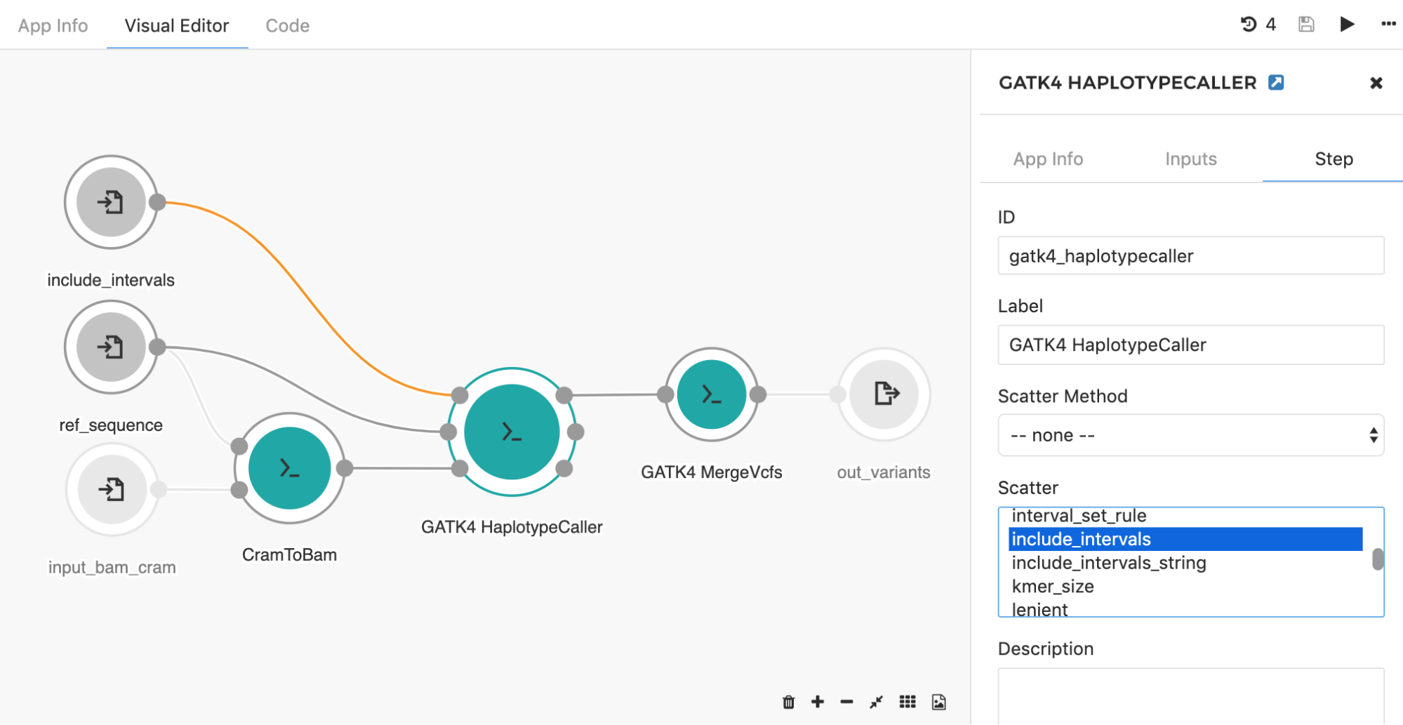
Another common application of the scatter feature is seen when using the HaplotypeCaller app to call SNPs and indels across large genomic intervals (e.g. entire chromosome set). Instead of searching through the whole genome, the HaplotypeCaller app has an option which allows for defining specific genomics regions (e.g. intervals) within which variants will be called. With this in mind, it is possible to set up the processing such that each chromosome is run independently from each other. This is a great example of a task that will benefit from scattering, as users can run the tool in parallel across all chromosomes. By choosing the “include_intervals” input from the Scatter box (Figure 8), the tool will perform scattering by the genomic intervals input, which will result in an independent job for each provided interval file (usually BED or TXT format which contains interval name along with the corresponding start and end genomic coordinates).
There are situations where it is desirable to create one job per multiple input files. To accomplish this, a way to bin the input files into a series of grouped items is needed. A good example of this is when an input sample has paired-end reads, and users want to create jobs for each sample, not each read. In this case, SBG Pair FASTQs by Metadata tool (available as a public app) can be used to create the group for each pair, and this tool should be inserted upstream of the tool on which you will apply scatter in your workflow.
Recalling the comparison between Batch Analysis and Scatter from the previous section, it may perhaps appear that these features are alternatives to one another. Even though they are intended for somewhat similar purposes, Scatter and Batch Analysis are mostly used as complementary features – they can be applied to the same analysis, such as the HaplotypeCaller example above. The workflow already contains the HaplotypeCaller tool which is scattered across intervals. If we run the workflow and batch by input_bam_cram input, we would be able to create an individual task for each BAM/CRAM input file.
It is worth mentioning that many workflows available from the Public Apps Gallery already contain scattered tools. Hence, if a batch task is executed with those workflows, it efficiently accomplishes parallelization on both levels – within the task (with Scatter) and across multiple instances (with Batch Analysis). One example of this is the Bismark Analysis workflow that takes raw reads (WGBS or RRBS) as inputs, performs sequence alignment, and outputs methylated sites. Prior to the alignment steps, low quality reads along with adapters are filtered out using the TrimGalore! tool that is not resource-intensive, but requires more time to do the work. To compensate for that, the reads were split into chunks and TrimGalore! was run in parallel for each chunk using Scatter. Doing so managed to significantly drop the time spent in this step, while utilizing all the available resources within the selected instance type. Unlike in the previous example where already-existing intervals were leveraged in order to enable parallelization, the pipeline goes one step further – pinpointing the app with a poor resource usage and inventing the logic that enables the application of Scatter. Finally, running this workflow in a batch mode will even further optimize the time spent for the analysis.
More details about all this topic can be found in the related blog post – Optimized Workflow for Bisulfite Sequencing Data Analysis.
Configuring default computational resources
In a previous section, this guide reviewed methods for controlling the computational resources from the task page, where you can choose an instance for the overall analysis on-the-fly. While in many cases this is the recommended method, customizing the workflow for a specific scenario or optimizing it with Scatter will sometimes require setting up default instance types. This can be configured from the tool/workflow editor by using the instance hint feature. This feature allows users to 1) select the appropriate resources for the individual steps (i.e. tools) in a workflow, and 2) define the default instance for the entire analysis (either a single app or a workflow).
The user who creates the analysis can choose to set the default instance if they are confident that their analysis will work well on a particular instance and they do not want to rely on the user settings or the platform scheduler. However, if the default instance is not set, the user can select the instance for the analysis from the task page (as described above), or the user can leave it to the platform scheduler to pick the right instance based on the resource requirements for the individual app(s).
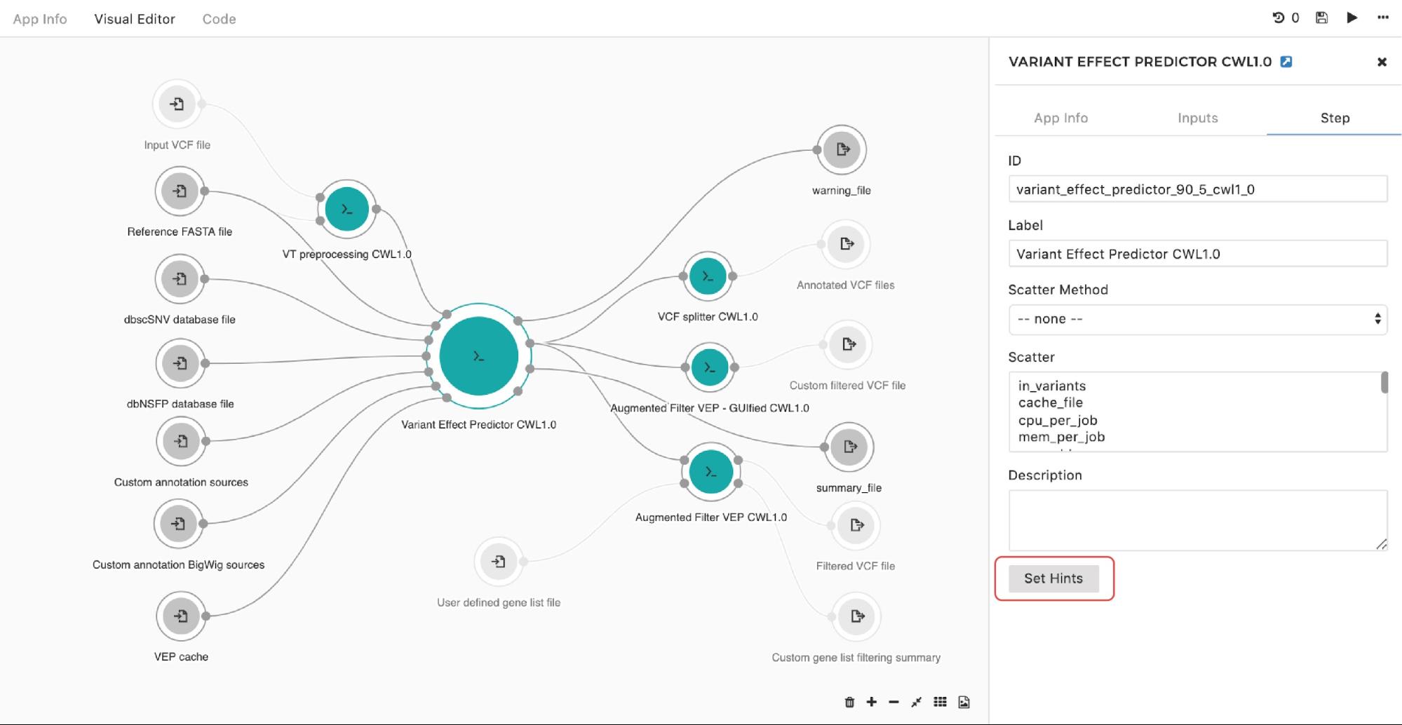
To set up an instance hint (i.e. chose a specific instance type) on the particular tool in the workflow, this can be done by entering the editing mode, then double-clicking on the node and selecting Set Hints button under the Step tab as follows:
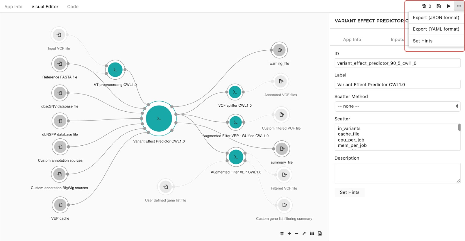
A configuration pop-up window will appear, then users can select instance types. This also applies for managing the instance hints for the whole workflow. The only difference is that we get to the pop-up window through the drop-down menu in the upper right corner in the editor as shown in Figure 10:
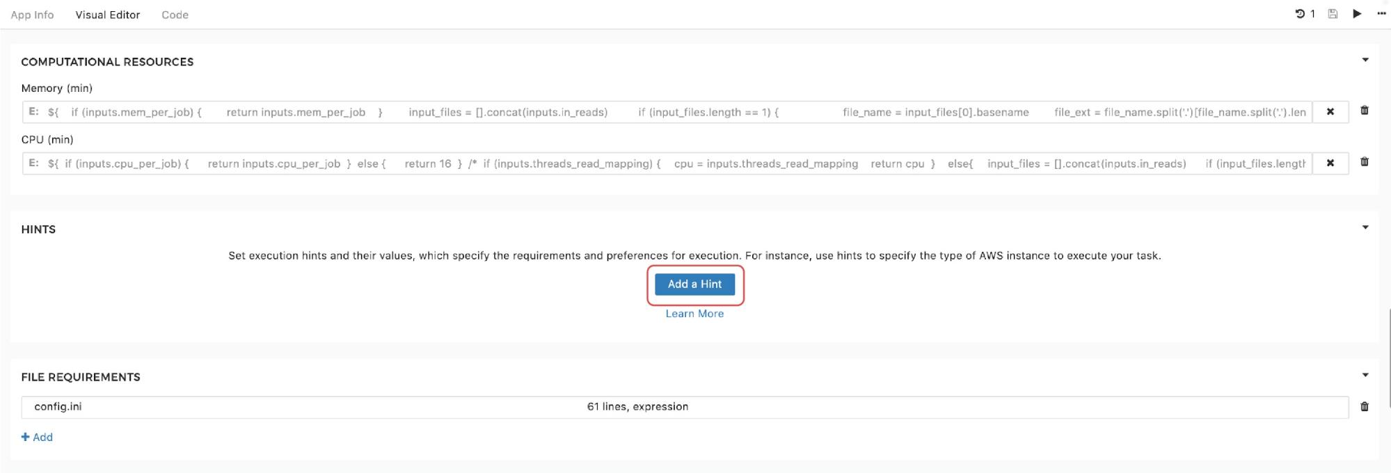
Finally, to set the instance hints for an individual app, edit the app and scroll down to the HINTS section shown in Figure 11:
Recalling the resource parameters description, you may wonder what happens if the resource parameters are set and an instance hint is configured within the same tool. In this case, the scheduler will prioritize the instance hint value and will allocate the instance based on that information. However, the information about resource parameters needed for one job is not completely ignored. Namely, if a workflow is about to be run, and the set-up is such that multiple jobs can be executed in parallel on the same instance (i.e. we use Scatter feature), resource parameters are also taken into consideration. These parameters are not used for the instance allocation, but they determine the number of different jobs that can be “packed” together for simultaneous runs on the given instance. A detailed explanation of the scatter feature that enables this is provided in a previous section.
Further analysis and interpretation of your Results
On the CGC, users can further analyze their data by leveraging Python notebooks or R interactive capabilities by using the Data Studio feature. With the Data Studio, users can easily access the files in their project for use in an R- or Python-based environment, without the need to download them to your local machine, and with the added flexibility of choosing computational resources.
Getting started
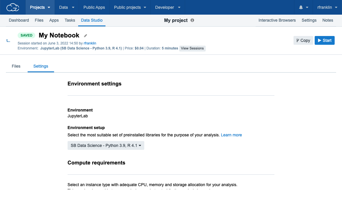
To access Data Studio:
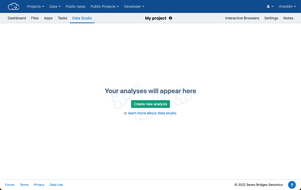
- Navigate to the Data Studio tab (Figure 12).
- Once on the following landing page, click the Create new analysis button which will start the analysis setup dialogue box (Figure 13)
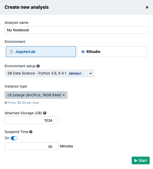
There are two computing environments available (Figure 13):
- JupyterLab
- RStudio
In this manual we will only focus on the JupyterLab environment. To learn more about RStudio, check out Data Studio documentation.
There are several Amazon Web Services (AWS) or Google instance types that users can choose from. If an AWS location was selected at the time of project creation, then users will see AWS instance options, likewise for when Google is set as the project location. It is shown in Figure 13 that there is a drop-down menu where users can configure the environment: meaning that users can choose one of two Docker images with pre-installed Python and R packages. The Seven Bridges default image contains the most common packages needed for scientific analysis and visualizations. In addition, Suspend time can be configured as a safety mechanism to enable automatic termination of the instance after a period with no activity. This feature can be turned off completely if a user plans a longer interaction and does not want to risk termination. We recommend that users carefully check the Location and Suspend Time settings before starting the analysis, especially if running an existing one which already has its own configuration (Figure 14).
After you set up the preferences, click the Start button to spin up the instance. It may take several minutes for the instance to initialize.
JupyterLab environment
Once the instance is ready, the editor will open automatically.
From there, users can move forward with their analysis (Figure 16):
Accessing the files
The files which users can analyze within the notebook are:
- files present in the analysis – either files uploaded directly in the analysis workspace (the home folder for the interactive analysis) or files produced by the interactive analysis itself, and
- files present in the project
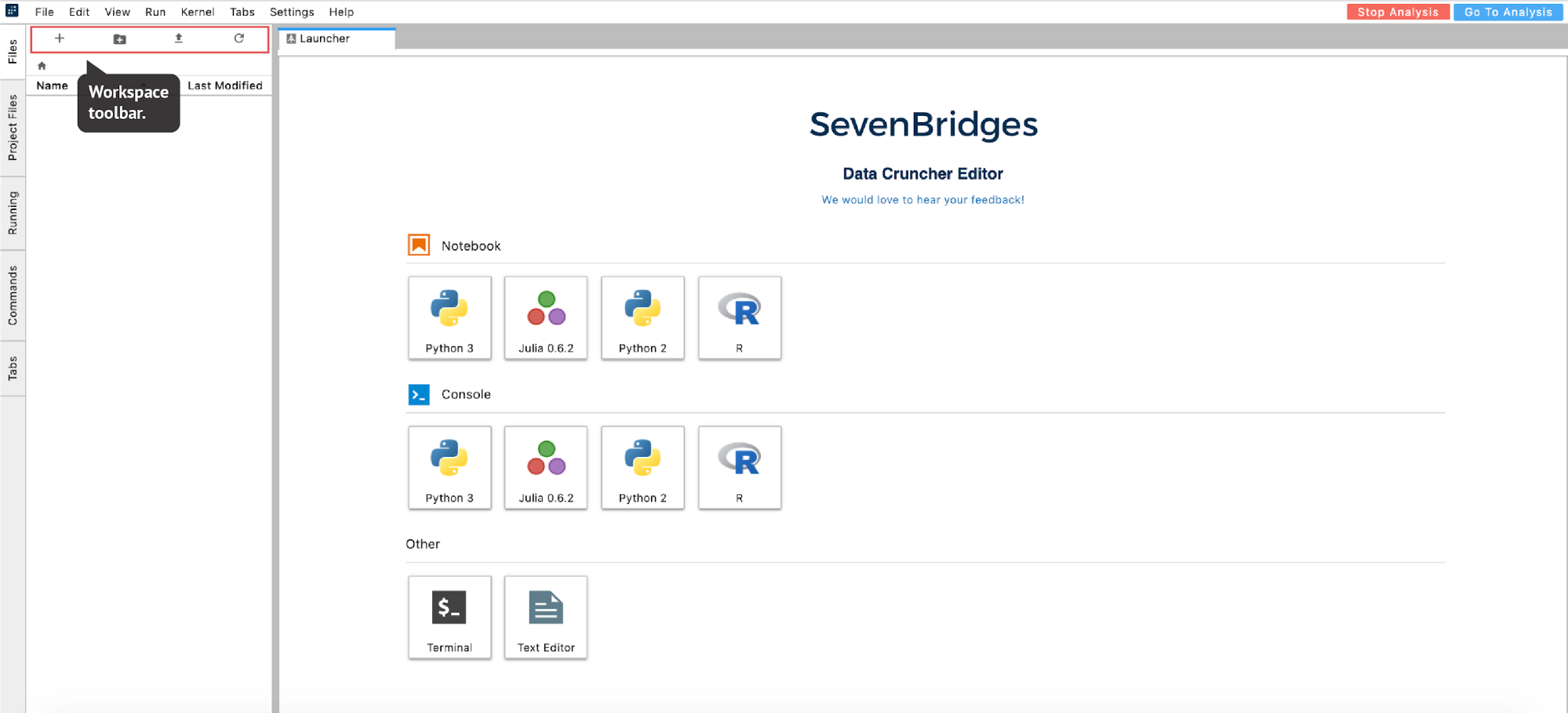
The list of files available in the analysis is displayed in the left-hand panel under the Files tab. This is a list of items in the /sbgenomics/workspace directory, which is the default directory for any work that users perform during a session. To control the content in this directory (create new folder, upload files etc.), users can utilize the workspace toolbar located above this panel (Figure 16).
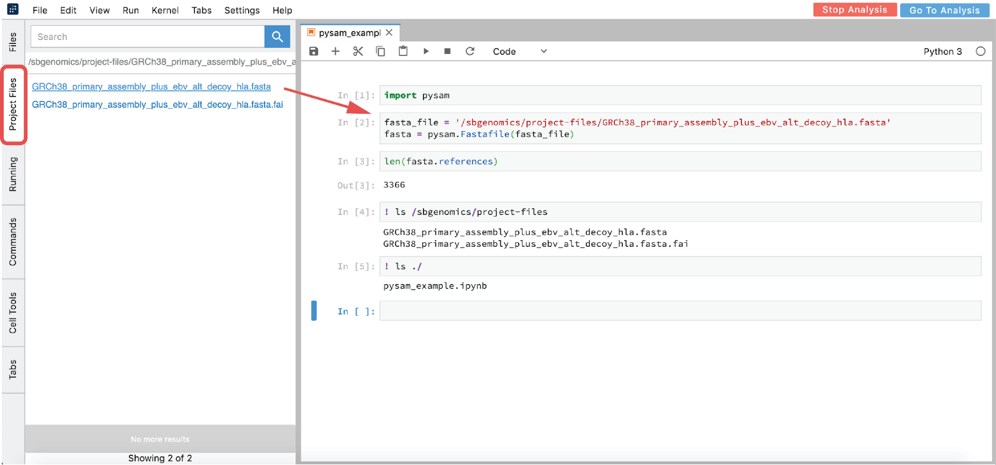
However, if you are interested in using an interactive analysis to access the data from your project, list all the files in the /sbgenomics/project-files directory and select the one of interest (see cell [4] in Figure 17).
- From GUI – click on the file you want to analyze in the Project Files tab (this action copies the path to clipboard) and paste the path in the notebook (Figure 17)
- List all the files in the
/sbgenomics/project-filesdirectory and select the one of interest in (see cell [4] in Figure 17).
This path is immutable across different projects. Therefore, if a user copies the analysis to another project and they have referenced their file this way, it will function the same way in the new project.
In the previous example, “!” was used in two notebook cells to switch from Python to shell interpreter, and hence denote that these cells should be executed as shell commands. If there is a need to use shell more intensively, (such as for installation purposes, etc), the notebook environment can become impractical. Fortunately, there is an option to mitigate this: a terminal can be opened from the launcher page (Figure 16).
Saving the created files
Finally, when the user has completed the analysis and wants to save the results to their project, the next step is to copy the files to the /sbgenomics/output-files directory from the terminal. Please note that only smaller files (e.g. .ipynb files) will continue to live in the analysis after it has stopped. Hence, all other needed files need to be saved before you decide to terminate the session.
RStudio Environment
For users who prefer to conduct their analysis using RStudio, they should follow the identical procedure from above (Figures 13 and 15) with an exception of instead selecting RStudio in the dialogue box shown in Figure 13.
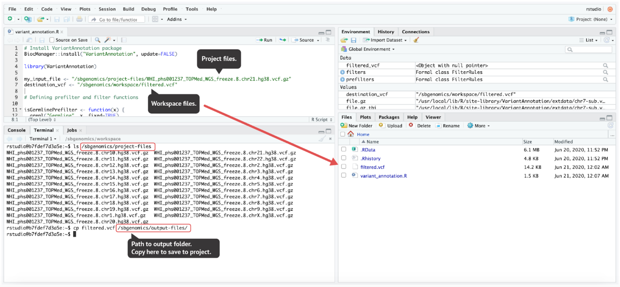
Accessing and saving the files in RStudio
Unlike the JupyterLab environment, RStudio environment does not offer convenient file handling from the GUI. However, the same paths that we mentioned in previous sections are also used in RStudio:
- Project files directory:
/sbgenomics/project-files - Workspace directory:
/sbgenomics/workspace - Output directory:
/sbgenomics/output-files
Further reading
Data Studio documentation:
About Data Studio
YouTube demo:
https://www.youtube.com/watch?v=LP53HNyG9gs&t=6m35s
Data Browser Essentials
The Seven Bridges platform enables users to also examine some of the most popular public cancer datasets, such as The Cancer Genome Atlas (TCGA). To deal with huge numbers of samples and files which are available within these datasets (TCGA has over 314,000 files), the Seven Bridges team has developed the Data Browser feature. The Data Browser enables users to visually explore, query and filter data by its metadata attributes.
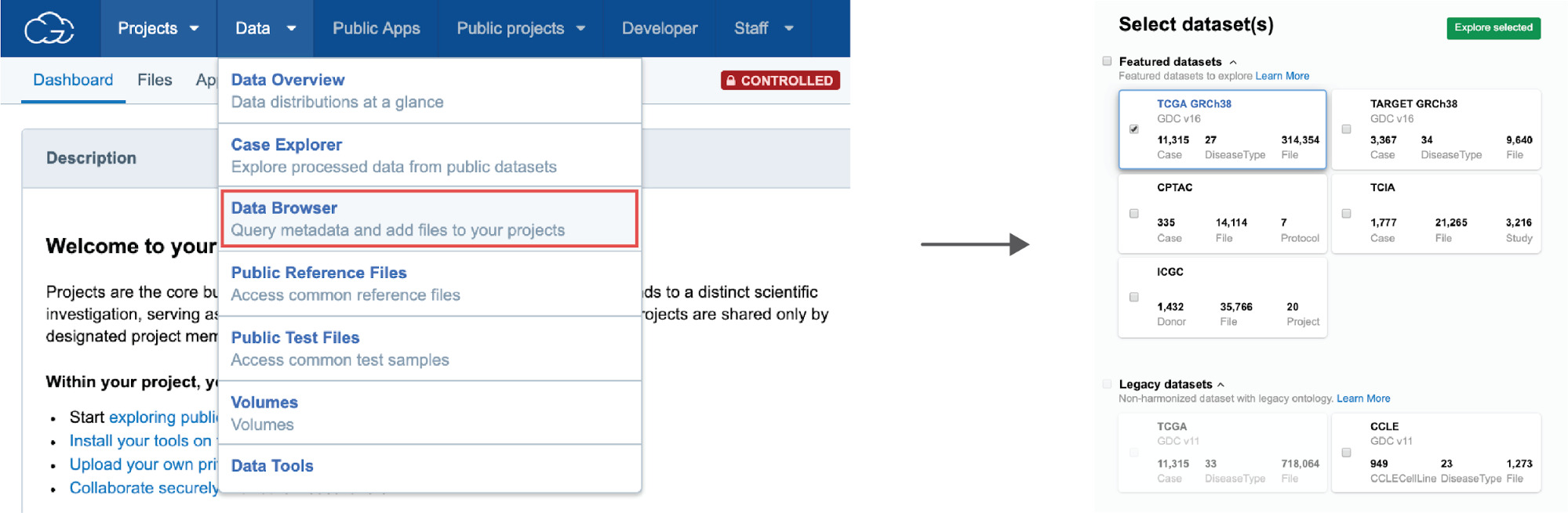
Quickstart
To get started with the Data Browser, users can go to the top navigation bar and choose Data Browser. Next, users will be prompted to select the dataset of interest, or to select multiple datasets for those interested in looking across multiple datasets at once.
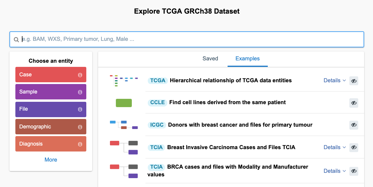
From here, users can proceed to query the dataset(s), explore previously saved queries, or check out the example queries (Figure 19). By typing in some of the known keywords in the search bar (e.g. Lung Adenocarcinoma, miRNA-seq, etc.) users can quickly filter through the data and get your first query building blocks.
The following section will focus on understanding how queries can be built from scratch and how users can get exactly what they need by using the Data Browser.
Data Browser Querying Logic
While the Data Browser is an effective tool for getting files of interest, there are a few aspects which could initially cause confusion. Different arrangements of the same query blocks may produce different results, which may be unexpected. Indeed, querying logic may seem confusing and overwhelming, but featured below are a few examples which will clarify the most essential functions. All examples use the TCGA GRCh38 dataset and represent querying from GUI.
To begin, here is a simple, intuitive example:
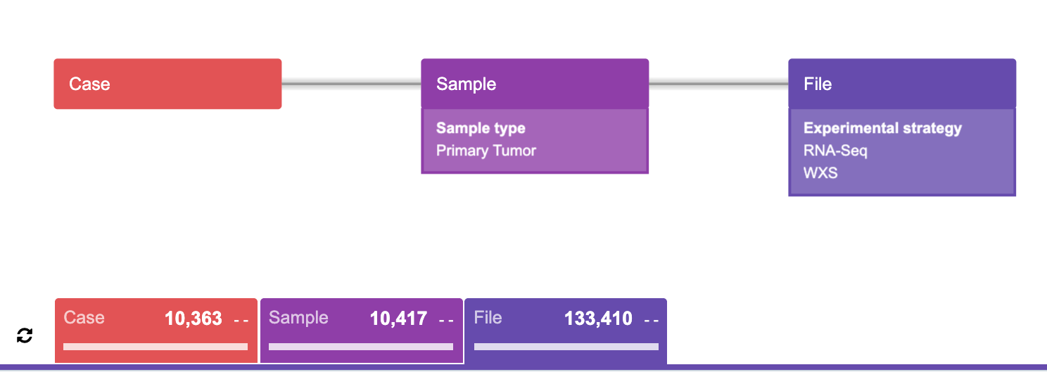
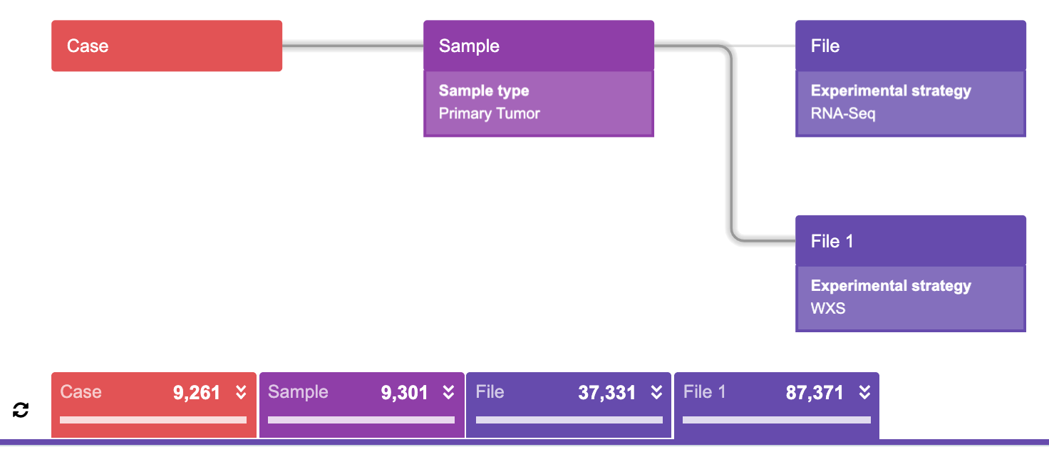
Most users will likely agree as to what this particular query (Figure 21) represents. To begin, try to translate this “diagram language” into words. The result of this query diagram would be:
“Find all the cases such that each case has at least one primary tumor sample which has at least one of EITHER RNA-Seq OR WXS experimental strategy file, then find the corresponding samples and the corresponding files.”
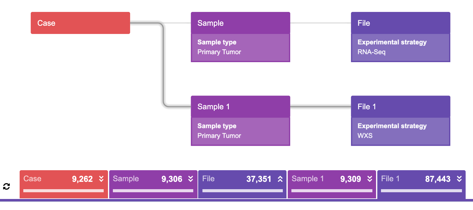
Next, examine a slightly different example:
A statement for this query would be something similar to:
“Find all the cases such that each case has at least one primary tumor sample which has at least one RNA-Seq AND at least one WXS experimental strategy file, then find the corresponding samples and the corresponding files.”
It is unusual for this parallel connection to represent the “AND” operation. To contrast, keep in mind that the “OR” operation is represented in the previous example. Correspondingly, the resulting numbers of files resulting from each query are greater in the first example, which uses an “OR” operation, then in the second example, which uses the “AND” operation.
Now examine a third option for a similar query:
This query represents the following statement:
“Find all the cases such that each case has at least one primary tumor sample which has at least one RNA-Seq experimental strategy file AND at least one primary tumor sample which has at least one WXS experimental strategy file, then find the corresponding samples and the corresponding files.”
This query is less intuitive to understand, but following the same logic as in the previous simpler queries, the correct result can still be deduced. The following evidence to support that this interpretation of the query is correct is as follows: taking a look at the returned counts below the graphs (Figure 21, 22), it is evident that these numbers are very similar. The reason for this lies in the fact that the majority of these samples do contain at least one file from each given category. To be precise, there is only one case among all cases returned in the third query that does not have both WXS and RNAseq experimental strategies in the same primary tumor sample.
Now that the Data Browser querying has been described in detail, this logic may be used to create a query which is a very common starting point for many bioinformatics analyses: finding matched tumor and normal samples.
The following is an example using TCGA Breast Invasive Carcinoma cohort (TCGA BRCA):
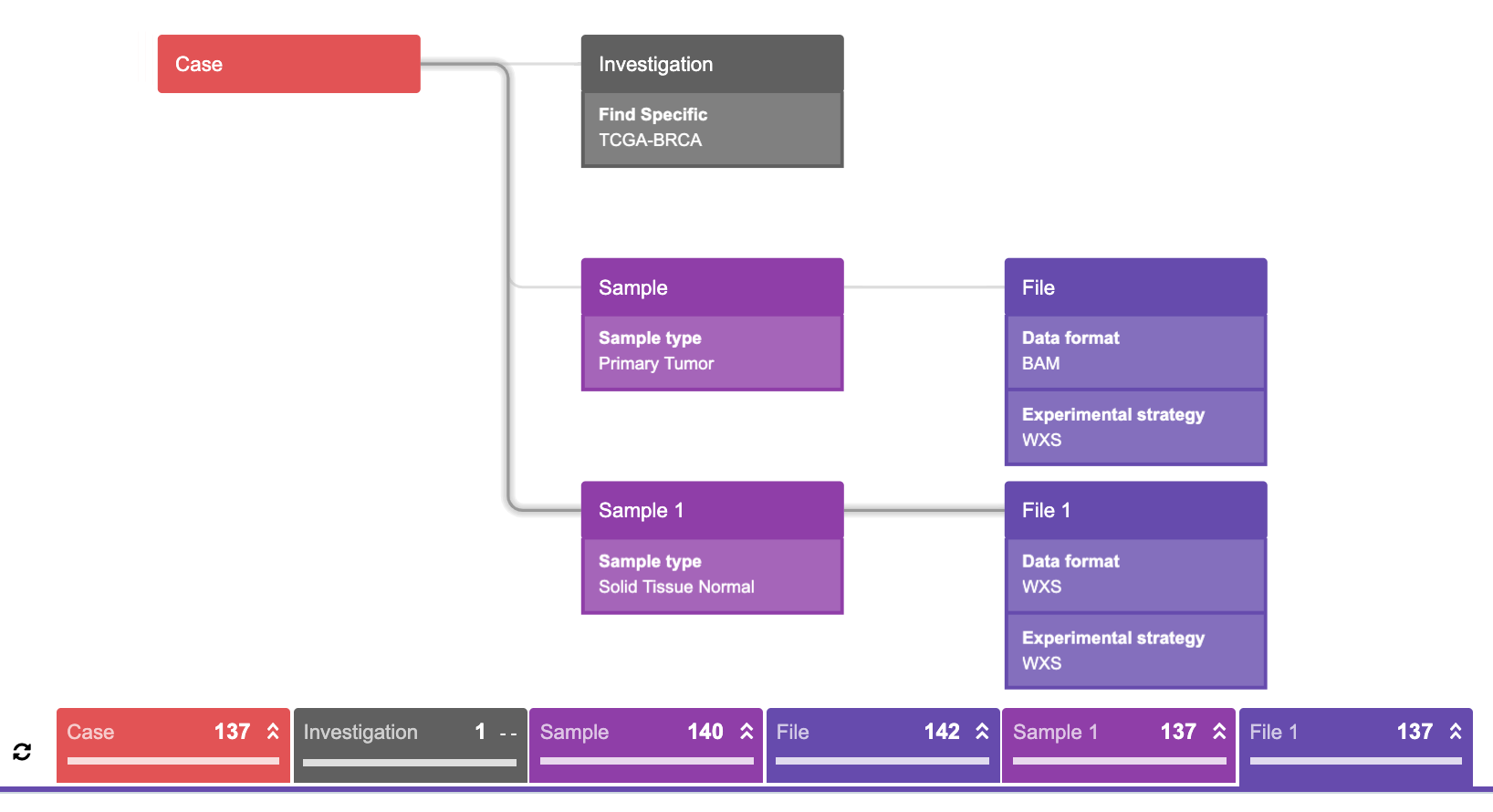
This query represents the following statement:
“Find all the cases such that each case has Breast Invasive Carcinoma (TCGA-BRCA) AND at least one primary tumor sample which has at least one WXS experimental strategy file in BAM format AND at least one solid tissue normal sample which has at least one WXS experimental strategy file in BAM format, then find the corresponding samples and the corresponding files.”
Simply put: each case needs to fulfill all three conditions in order to be pulled out (hence three branches).
It is important to mention that when copying files into a project, BAI files will be copied together with the BAM files automatically, so users do not need to worry about finding the associated index files. Also, a users will not be billed for keeping these public files in your project (as explained in subsequent sections). However, the storage for any derived files (e.g., FASTQ files derived from BAM files) will be charged.
Computational Limits
Before deciding to run a large number of simultaneous tasks, it is good to take a moment to learn more about platform limitations.
Because the Amazon account used for Cancer Genomics Cloud comes with a limit on the number of instances that can be allocated at the same time, we were forced to impose restrictions on the maximum number of running tasks per user. By doing so, we are securing the computational resources availability on the platform at any given time, and making sure that the users seeking highly parallelized analysis do not block all other users. This limit is currently set to 80 parallel tasks. In other words, if a user creates a project and triggers a batch analysis containing 100 tasks, they will get 80 running tasks whereas the remaining 20 tasks will have a “QUEUED” status until some of the 80 tasks finish.
If you need to run at a higher throughput, we would highly appreciate you reaching out to our team, so we can work together to find the best solution.
Storage Pricing
When you copy the files from the CGC data sets, TCGA or TARGET, to your project, you will not be charged for storing those files. The files from these publicly available datasets are located in a cloud bucket maintained by NCI’s Genomic Data Commons (GDC). These files are only referenced in your project, while the physical file remains in the GDC.
A similar logic applies to all files: if you copy a file from one project to another, that file is only referenced in the second project, without creating a physical copy and without additional storage expenses. This also means that if you create multiple copies and then delete the original file, the copies will still remain and the file will still accrue storage costs until ALL copies are deleted.
In addition to computation, storage costs are made up of the cost for storing derived files or any files that you have uploaded. It is important to note that this applies as long as the users keep the files in their projects. To minimize storage costs, it is recommended to check on user files after each project phase is completed and discard any files which are not needed for the future analysis. Note that intermediate files can always be recreated by running the analysis again, and that the cost to re-create these files can sometimes be less than storing the files in the project. As noted in the previous paragraph, multiple copies of a file are charged only once. Consequently, when deleting files which have a copy in other projects, users will still accrue storage expenses until all the copies are removed.
If you have questions about moving your files to manage storage costs, please contact us at [email protected] to learn more about streamlining the process. For more information about storage and computational pricing, visit our Knowledge Center.
Appendix
Using the API
There are numerous use cases in which users might want to have more control over their analysis flow, or simply want to automate custom, repetitive tasks. Even though there are a lot of features enabled through the platform GUI, certain types of actions will benefit from using the API.
In the section below, a couple of API Python code snippets are provided for the purpose of this manual. These code snippets have proven to be useful for mitigating most frequent obstacles when running large scale analyses on the Cancer Genomics Cloud.
Before you proceed, note that all examples are written in Python 3.
Install and configure
To be able to run Seven Bridges API, users should first install sevenbridges-python package:
pip install sevenbridges-python
After that, users can then experiment with some basic commands, just to get a sense of how the Seven Bridges API works. To be able to initialize the sevenbridges library, each user will need to generate their authentication token and plug it into the following code:
import sevenbridges as sbg
api = sbg.Api(url='https://cgc-api.sbgenomics.com/v2', token='')Managing tasks
Here is a simple code for fetching all task IDs from a given project and printing the status metrics:
import collections

# First you need to provide project slug from its URL:
test_project = 'username/project_name'

# Query all the tasks in the project
# Query commands may be time sensitive if there is a huge number of expected items
# See explanation below
tasks = api.tasks.query(project=test_project).all()
statuses = [t.status for t in list(tasks)]

# counter method counts the number of different elements in the list
counter = collections.Counter(statuses)
for key in counter:
    print(key, counter[key])
The previous code should result in an output similar to this:
ABORTED 1
COMPLETED 8
FAILED 1
DRAFT 1
In order to fully understand this section, it is vital to provide an explanation of API rate limits.
The maximum number of API requests, i.e. commands performed on the api object, is 1000 requests in 5 minutes (300 seconds). An example of this command is the following line from the previous code snippet:
tasks = api.tasks.query(project=test_project).all()By default, 50 tasks will be fetched in one request. However, the maximum number is 100 tasks and it can be configured as follows:
tasks = api.tasks.query(project=test_project, limit=100).all()In other words, users typically would have to wait for the renewed requests for a couple of minutes if the project contained more than 100,000 tasks. This scenario almost never happens in practice because it is unusual to have this number of tasks in one project. However, this number can be easily reached for the project files to which the same rule applies. The next few code examples illustrate handling files.
Managing files
In this section, methods to perform some simple actions on the project files are described. The following code will print out the number of files in the project:
files = api.files.query(project=test_project, limit=100).all()
len(list(files))
In order to now read the metadata of a specific file, the following code can be run:
files = api.files.query(project=test_project, limit=100).all()
for f in list(files):
    if f.name == '95622ade-3084-4ddb-93a1-e6baac7769f7.htseq.counts.gz':
        my_meta = f.metadata
        for key in my_meta:
            print(key,':', my_meta[key])
The output will appear similar to this:
sample_uuid : fed73c89-75f1-45c9-b14b-7840c52c305f
gender : female
vital_status : dead
case_uuid : d63c186d-add6-492e-8250-e83f46d39d00
disease_type : Bladder Urothelial Carcinoma
aliquot_uuid : 024bc00e-0419-4dc6-8df4-ad3af476314d
aliquot_id : TCGA-DK-A3WX-01A-22R-A22U-07
age_at_diagnosis : 67
sample_id : TCGA-DK-A3WX-01A
race : white
primary_site : Bladder
platform :
sample_type : Primary Tumor
experimental_strategy : RNA-Seq
days_to_death : 321
reference_genome : GRCh38.d1.vd1
case_id : TCGA-DK-A3WX
investigation : Bladder Urothelial Carcinoma
ethnicity : not hispanic or latino
As previously mentioned, the majority of publicly available datasets have immutable metadata. However, if a user has their own files and want to add or modify metadata, they can do so by using the following template:
files = api.files.query(project=test_project, limit=100).all()
for f in list(files):
    if f.name == 'example.bam':
        f.metadata['foo'] = 'bar'
        f.save()
        my_meta = f.metadata
        for key in my_meta:
print(key,':', my_metadata[key])Bulk operation: reducing the number of requests
By inspection, it is evident that f.save() is called each time it is desired to update the file with new information. This means that the new API request is generated, and recalling that there is a limit of 1,000 requests in 5 minutes, it is evident that this number is easily reached. To solve this issue, bulk methods are used:
all_files = api.files.query(project=test_project, limit=100).all()
all_fastqs = [f for f in all_files if f.name.endswith('.fastq')]
changed_files = []

for f in all_fastqs:
    if f is not None:
        f.metadata['foo'] = 'bar'
        changed_files.append(f)

if changed_files:
    changed_files_chunks = [changed_files[i:i + 100] for i in range(0, len(changed_files), 100)]
    for cf in changed_files_chunks:
        api.files.bulk_update(cf)
In this example, it was elected to set metadata only for the FASTQ files found within the project. This was performed by triggering only one API request per 100 files – first splitting the list of files into chunks of at most 100 files, and then running the api.files.bulk_update() method on each chunk.
For more information about other useful bulk operations, see this section in the API Python documentation.
Managing batch tasks
Another vital topic to discuss is batch analysis handling. If there had been batch tasks in the project used for printing out task status information in one of the previous examples, the output would not have included metrics which include children tasks statuses as well. To be able to query children tasks, a couple of additions to the API code is needed.
First, a method to check which tasks are batch tasks:
test_project = 'username/project_name'
tasks = api.tasks.query(project=test_project).all()
for task in tasks:
    if task.batch:
        print(task.name)
Typically, users will want to automatically rerun the failed tasks within batch analysis. The following method described how to filter out failed tasks for the given batch analysis and rerun those tasks with an updated app:
test_project = 'username/project_name'
my_batch_id = 'BATCH_ID'
my_batch_task = api.tasks.get(my_batch_id)
batch_failed = list(api.tasks.query(project=test_project,
                                        parent=my_batch_task.id,
                                        status='FAILED',
                                        limit=100).all())
print('Number of failed tasks: ', len(batch_failed))

for task in batch_failed:
    old_task = api.tasks.get(task.id)
    api.tasks.create(name='RERUN - ' + old_task.name,
                     project=old_task.project,
                     # App example: cgcuser/demo-project/samtools-depth/8
                     # You can copy this string from the app's URL
                     app=api.apps.get('username/project_name/app_name/revision_number'),
                     inputs=old_task.inputs,
                     run=True)
    print('Running: RERUN - ' + old_task.name)
As shown above, there is no need to specify inputs for each task separately – those inputs can be n automatically passed from the old tasks. However, this only relates to re-running the tasks in the same project. If a user desires to re-run the tasks in a different project, they will need to write a couple of additional lines to copy the files and apps.
Collecting specific outputs
The following example is a useful reference for users who have had their analysis completed successfully and wish to fetch and examine further specific outputs. Detailed below is the code for copying all the files belonging to a particular output node from all successful runs to another project. The code can be easily modified to fit a specific purpose, e.g. renaming the files, deleting them if desired to offload the storage, providing those as inputs to another app, etc. The code may appear complex because it contains error handling and logging, but the iteration through the tasks and collecting the files of interest is fairly simple.
The resulting code will look like this:
import sevenbridges as sbg
import time
from sevenbridges.http.error_handlers import (rate_limit_sleeper, maintenance_sleeper, general_error_sleeper)
import logging

logging.basicConfig(level=logging.INFO)
time_start = time.time()
my_token = '<INSERT_TOKEN>'
# Copy project slug from the project URL
my_project = 'username/project_name'
# Get output ID from the "Outputs" tab within "Ports" section on the app page
my_output_id = 'output_ID'
api = sbg.Api('https://cgc-api.sbgenomics.com/v2', token=my_token, advance_access=True,
              error_handlers=[rate_limit_sleeper, maintenance_sleeper, general_error_sleeper])

tasks_queried = list(api.tasks.query(project=my_project, limit=100).all())
task_files_list = []
print('Tasks fetched: ', time.time() - time_start)
for task in tasks_queried:
    if task.batch:
        ts = time.time()
        children = list(api.tasks.query(project=my_project,
                                        parent=task.id,
                                        status='COMPLETED',
                                        limit=100).all())
        print('Query children tasks', time.time() - ts)
        for t in children:
            task_files_list.append(t.outputs[my_output_id])
    elif task.status == 'COMPLETED':
        task_files_list.append(task.outputs[my_output_id])

print('Outputs from all tasks collected: ', time.time() - time_start, '\n')
fts = time.time()

for f in task_files_list:
    print('Copying: ', f.name)
    # Uncomment the following line if everything works as expected after inserting your values
    # f.copy(project='username/destination_project')

print('\nAll files copied :', time.time() - fts)
print('All finished: ', time.time() - time_start)
There are two major cases – (1) either users run into the batch task in which case it is required to iterate through all completed children tasks, or (2) users simply run into an individual task and only need to check if the status is “COMPLETED”. If any of these two conditions are satisfied, then the output of interest is collected (lines 19 to 30) and then loop through those to copy the files (lines 35 to 38).
If you have any questions or need help with using the API, feel free to contact our support.